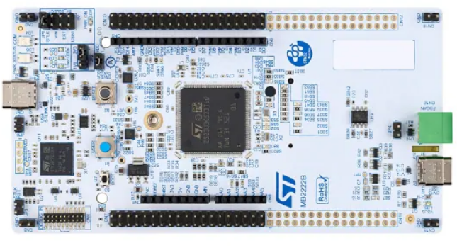
1.1 STM32U3C5 与 HSP 硬件信号处理器

STM32U3C5ZIT6Q 是意法半导体推出的超低功耗微控制器，搭载 Arm Cortex-M33 内核（最高 96 MHz ），配备 2 MB Flash 和 640 KB RAM

2.1 硬件清单

NUCLEO-U3C5ZI-Q 集成 STM32U3C5ZIT6Q USB Type-C 数据线 | 供电、调试、串口通信 LSM6DSO16IS (板载) 或外接加速度计 采集三轴加速度数据 精密万用表或 STM32CubeMonitor-Power IDD 功耗测量 (可选) NUCLEO-U3C5ZI-Q 板载了 STLINK-V3EC 调试器，支持 SWD 调试和虚拟串口（VCP），默认波特率 115200。板上 JP5（IDD measurement）跳线专门用于测量 STM32 微控制器的电流消耗，这是后续功耗测试的关键接口。

2.2 软件工具链

Python TensorFlow STM32CubeProgrammer STM32CubeMonitor-PowerSTM32CUBEMX STM32CUBIDE

Python 环境建议通过 Anaconda 创建独立环境：

conda create -n stm32ai python=3.10 conda activate stm32ai pip install tensorflow==2.15.0 numpy pandas matplotlib scikit-learn

2.3 ST Edge AI CLI 路径确认

安装 X-CUBE-AI 后，stedgeai.exe（Windows）或 stedgeai（Linux/macOS）位于以下路径： plain

Windows

C:\Users<用户名>\STM32Cube\Repository\Packs\STMicroelectronics\X-CUBE-AI<版本>\Utilities\windows\stedgeai.exe

三、人体行为识别模型训练

3.1 数据集准备

人体行为识别（HAR）使用三轴加速度计数据作为输入。本教程采用经典的 UCI HAR Dataset（基于智能手机采集的 6 类活动数据），你也可以使用自定义数据集。 数据采集参数： 采样率：50 Hz（每秒 50 个样本） 传感器：三轴加速度计（X, Y, Z） 活动类别：Walking、Walking Upstairs、Walking Downstairs、Sitting、Standing、Laying 窗口大小：2.56 秒（128 个采样点） 滑动步长：50% 重叠（64 个采样点） FFT 预处理参数（关键配置，决定 CNN 输入形状）： FFT 点数：256 点（补零至 256 点） 输出频谱范围：保留前 128 个频率分量（幅度谱） 三轴合并：将 X/Y/Z 三轴频谱堆叠为 3 通道输入 CNN 输入张量形状：(1, 128, 3) —— 128 个频率 bin，3 个通道（对应 X/Y/Z 轴）

3.2 数据预处理与 FFT 转换

以下 Python 代码实现从原始加速度计数据到 FFT 频谱图的转换，包含必要的错误检查： Python import numpy as np import tensorflow as tf from scipy.fft import fft import os

============ 配置参数 ============

SAMPLE_RATE = 50 # 采样率 Hz WINDOW_SIZE = 128 # 窗口大小 (2.56s @ 50Hz) STRIDE = 64 # 滑动步长 (50% 重叠) FFT_SIZE = 256 # FFT 点数 NUM_AXES = 3 # 三轴加速度计 (X, Y, Z) NUM_CLASSES = 6 # 活动类别数

标签映射

ACTIVITY_LABELS = ['Walking', 'Walking_Up', 'Walking_Down', 'Sitting', 'Standing', 'Laying']

def extract_fft_features(accel_data): """ 将三轴加速度计时域数据转换为 FFT 频谱特征 参数: accel_data: shape (N, 3) —— N 个时间点的三轴数据 返回: fft_features: shape (128, 3) —— 频谱幅度特征 """ if accel_data.shape[1] != NUM_AXES: raise ValueError(f"Expected {NUM_AXES} axes, got {accel_data.shape[1]}") fft_features = np.zeros((FFT_SIZE // 2, NUM_AXES), dtype=np.float32)

for axis in range(NUM_AXES): signal = accel_data[:, axis]

应用 Hann 窗减少频谱泄漏

window = np.hanning(len(signal)) windowed = signal * window

执行 FFT

fft_result = fft(windowed, n=FFT_SIZE)

取幅度谱的前半部分 (0-25Hz)

magnitude = np.abs(fft_result[:FFT_SIZE // 2])

归一化，避免除零

max_val = np.max(magnitude) if max_val == 0: fft_features[:, axis] = 0.0 else: fft_features[:, axis] = magnitude / max_val

return fft_features

def create_windows(data, labels, window_size=128, stride=64): """ 使用滑动窗口切分时间序列数据 """ if len(data) < window_size: raise ValueError(f"Data length {len(data)} is less than window_size {window_size}") windows = [] window_labels = []

for i in range(0, len(data) - window_size + 1, stride): window = data[i:i + window_size]

对每个窗口执行 FFT

fft_feat = extract_fft_features(window) windows.append(fft_feat)

使用窗口中点的标签

label_idx = min(i + window_size // 2, len(labels) - 1) window_labels.append(labels[label_idx])

return np.array(windows, dtype=np.float32), np.array(window_labels)

============ 加载 UCI HAR 数据集 ============

def load_uci_har_dataset(base_dir='./UCI_HAR_Dataset/'): """加载并预处理 UCI HAR 数据集，包含文件存在性检查""" def load_txt(filepath): if not os.path.exists(filepath): raise FileNotFoundError(f"Dataset file not found: {filepath}") return np.loadtxt(filepath)

训练数据路径

train_dir = os.path.join(base_dir, 'train', 'Inertial Signals') test_dir = os.path.join(base_dir, 'test', 'Inertial Signals')

加载三轴训练数据

acc_x_train = load_txt(os.path.join(train_dir, 'total_acc_x_train.txt')) acc_y_train = load_txt(os.path.join(train_dir, 'total_acc_y_train.txt')) acc_z_train = load_txt(os.path.join(train_dir, 'total_acc_z_train.txt')) y_train = load_txt(os.path.join(base_dir, 'train', 'y_train.txt')) - 1 # 0-indexed

加载三轴测试数据

acc_x_test = load_txt(os.path.join(test_dir, 'total_acc_x_test.txt')) acc_y_test = load_txt(os.path.join(test_dir, 'total_acc_y_test.txt')) acc_z_test = load_txt(os.path.join(test_dir, 'total_acc_z_test.txt')) y_test = load_txt(os.path.join(base_dir, 'test', 'y_test.txt')) - 1

合并为 (samples, timesteps, 3)

train_data = np.stack([acc_x_train, acc_y_train, acc_z_train], axis=-1) test_data = np.stack([acc_x_test, acc_y_test, acc_z_test], axis=-1)

return train_data, y_train, test_data, y_test

加载数据

try: train_data, y_train, test_data, y_test = load_uci_har_dataset() except FileNotFoundError as e: print(f"Error: {e}") print("Please download the UCI HAR Dataset and place it in ./UCI_HAR_Dataset/") exit(1)

创建 FFT 窗口特征

try: X_train_fft, y_train_win = create_windows(train_data, y_train) X_test_fft, y_test_win = create_windows(test_data, y_test) except Exception as e: print(f"Error during feature extraction: {e}") exit(1)

print(f"训练集 FFT 特征形状: {X_train_fft.shape}") # (N, 128, 3) print(f"测试集 FFT 特征形状: {X_test_fft.shape}")

3.3 设计轻量级 CNN 模型

针对 STM32U3C5 的资源限制（640 KB RAM，2 MB Flash），需要设计一个足够轻量的 CNN。以下模型参数量约 15-30K，完全适配目标硬件，代码中加入输入形状校验： Python def create_har_cnn_model(input_shape=(128, 3), num_classes=6): """ 创建适用于 HSP 加速的轻量级 CNN 模型 设计原则:

• 仅使用 HSP 支持的层类型: Conv2D, MaxPool2D, AvgPool2D, Dense
• 避免 BatchNormalization（量化兼容性考虑）
• 控制参数量 < 50KB (INT8 量化后) """ if len(input_shape) != 2 or input_shape[0] <= 0 or input_shape[1] <= 0: raise ValueError("input_shape must be a tuple of two positive integers (height, channels)")

model = tf.keras.Sequential([ tf.keras.layers.Input(shape=input_shape), tf.keras.layers.Reshape((input_shape[0], input_shape[1], 1)),

第一个卷积块

tf.keras.layers.Conv2D(8, (3, 3), activation='relu', padding='same'), tf.keras.layers.MaxPooling2D((2, 2)), # 输出形状 (64, 2, 8) 假设输入128x3

第二个卷积块

tf.keras.layers.Conv2D(16, (3, 3), activation='relu', padding='same'), tf.keras.layers.MaxPooling2D((2, 2)), # (32, 1, 16)

第三个卷积块

tf.keras.layers.Conv2D(32, (3, 3), activation='relu', padding='same'), tf.keras.layers.MaxPooling2D((2, 2)), # (16, 1, 32)

展平 + 全连接

tf.keras.layers.Flatten(), tf.keras.layers.Dense(64, activation='relu'), tf.keras.layers.Dropout(0.3), tf.keras.layers.Dense(num_classes, activation='softmax') ])

return model

try: model = create_har_cnn_model() except Exception as e: print(f"Model creation failed: {e}") exit(1)

model.compile( optimizer=tf.keras.optimizers.Adam(learning_rate=0.001), loss='sparse_categorical_crossentropy', metrics=['accuracy'] )

打印模型结构

model.summary()

训练模型

history = model.fit( X_train_fft, y_train_win, validation_split=0.2, epochs=50, batch_size=32, callbacks=[ tf.keras.callbacks.EarlyStopping(patience=10, restore_best_weights=True), tf.keras.callbacks.ReduceLROnPlateau(factor=0.5, patience=5) ] )

评估测试集

test_loss, test_acc = model.evaluate(X_test_fft, y_test_win) print(f"测试集准确率: {test_acc:.4f}") if test_acc < 0.80: print("Warning: Accuracy is lower than expected. Consider adjusting model or training parameters.") 模型设计要点： 输入形状 (128, 3, 1) 对应 128 个频率 bin、3 轴（X/Y/Z）、1 通道灰度。 仅使用 Conv2D、MaxPooling2D、Dense —— 这些层类型均被 HSP 硬件支持。 避免使用 BatchNormalization —— 虽然 HSP 支持，但会增加量化复杂度；如需使用，建议放在 MaxPool 之后。 避免使用 DepthwiseConv2D —— 除非确定 HSP 版本支持（STEdgeAI-Core 4.0+ 已支持）。

四、模型量化（Post-Training Quantization）

4.1 INT8 量化的必要性

HSP 硬件加速器仅支持 8-bit 量化模型。浮点模型（float32）虽然可以通过 STM32Cube.AI 转换，但会回退到 CPU 执行，无法利用 HSP 加速，且推理速度和内存占用都显著劣于 INT8 模型。 量化将 float32 权重和激活值映射到 int8 范围（-128 到 127），带来 4 倍模型体积缩减和显著的推理加速。精度损失通常在 0.5% - 2% 范围内，对于大多数 HAR 任务可接受。

4.2 使用 TFLite Converter 进行 PTQ

以下代码执行完整的训练后量化（Post-Training Quantization），生成 HSP 兼容的 INT8 TFLite 模型，并包含量化误差的校验步骤： Python import tensorflow as tf import numpy as np

def representative_dataset(): """ 代表性数据集生成器 —— 用于 INT8 量化校准 重要: 必须使用与训练/测试数据分布一致的真实样本， 不能使用随机数据！建议选取 100-500 个代表性样本。 """ if len(X_train_fft) == 0: raise RuntimeError("Training data is empty, cannot create representative dataset.")

从训练集中选取 200 个样本用于校准

num_calib = min(200, len(X_train_fft)) calibration_indices = np.random.choice( len(X_train_fft), size=num_calib, replace=False ) for idx in calibration_indices: sample = X_train_fft[idx].astype(np.float32)

添加 batch 维度: (128, 3) -> (1, 128, 3)

yield [np.expand_dims(sample, axis=0)]

============ TFLite INT8 量化转换 ============

converter = tf.lite.TFLiteConverter.from_keras_model(model)

启用默认优化（包含量化）

converter.optimizations = [tf.lite.Optimize.DEFAULT]

设置代表性数据集（PTQ 必需）

try: converter.representative_dataset = representative_dataset except Exception as e: print(f"Failed to set representative dataset: {e}") exit(1)

强制使用纯 INT8 算子（关键！确保 HSP 能加速）

converter.target_spec.supported_ops = [ tf.lite.OpsSet.TFLITE_BUILTINS_INT8 ]

设置输入/输出数据类型为 int8

converter.inference_input_type = tf.int8 converter.inference_output_type = tf.int8

执行转换

try: tflite_model = converter.convert() except Exception as e: print(f"Conversion failed: {e}") exit(1)

保存量化模型

model_path = 'har_model_int8.tflite' with open(model_path, 'wb') as f: f.write(tflite_model)

验证模型文件已生成

import os if not os.path.exists(model_path): raise RuntimeError("TFLite model file was not created.")

model_size = os.path.getsize(model_path) print(f"INT8 量化模型大小: {model_size / 1024:.2f} KB") print(f"原始 FP32 模型大小估算: {model_size * 4 / 1024:.2f} KB")

============ 验证量化模型精度 ============

try: interpreter = tf.lite.Interpreter(model_path=model_path) interpreter.allocate_tensors() except Exception as e: print(f"Failed to load TFLite model: {e}") exit(1)

input_details = interpreter.get_input_details() output_details = interpreter.get_output_details()

获取量化参数

if len(input_details[0]['quantization_parameters']['scales']) == 0: raise RuntimeError("Model does not contain quantization parameters. Conversion may have failed.") input_scale = input_details[0]['quantization_parameters']['scales'][0] input_zero_point = input_details[0]['quantization_parameters']['zero_points'][0] print(f"输入量化参数: scale={input_scale:.6f}, zero_point={input_zero_point}")

测试量化模型准确率

correct = 0 total = len(X_test_fft) if total == 0: raise RuntimeError("Test set is empty.")

for i in range(total):

量化输入: float -> int8

input_data = (X_test_fft[i] / input_scale + input_zero_point).astype(np.int8) input_data = np.expand_dims(input_data, axis=0)

interpreter.set_tensor(input_details[0]['index'], input_data) interpreter.invoke() output = interpreter.get_tensor(output_details[0]['index'])

pred = np.argmax(output) if pred == y_test_win[i]: correct += 1

quant_acc = correct / total print(f"量化模型测试准确率: {quant_acc:.4f}") print(f"量化精度损失: {(test_acc - quant_acc) * 100:.2f}%") if (test_acc - quant_acc) > 0.03: print("Warning: Accuracy loss exceeds 3%. Consider using a larger calibration set or adjusting the model.") 关键注意事项： representative_dataset 不可省略 —— 若省略，转换器会退回到动态范围量化（权重 INT8，激活 float），HSP 将无法加速。 TFLITE_BUILTINS_INT8 必须唯一指定 —— 混合算子集会导致部分层在 CPU 上执行。 输入/输出设置为 tf.int8 —— 与 HSP 硬件数据格式匹配，避免运行时类型转换开销。

4.3 量化模型验证清单

表格 检查项 | 预期结果 | 验证方法 模型文件大小 | 原始模型的 1/4 左右 | os.path.getsize() 输入数据类型 | int8 | interpreter.get_input_details() 输出数据类型 | int8 | interpreter.get_output_details() 算子类型 | 均为 INT8 内核 | Netron 可视化工具 精度损失 | < 3% | 对比 FP32 与 INT8 测试准确率

五、STM32Cube.AI 模型生成（HSP vs CPU 模式）

5.1 使用 ST Edge AI CLI 生成模型代码

STEdgeAI-Core 的代码生成器将 TFLite 模型转换为高度优化的 C 代码，支持自动选择 HSP 加速层。生成两组代码：HSP 使能版本和纯 CPU 版本，用于后续对比测试。

5.1.1 生成 HSP 加速版本

bash

HSP 使能版本 (--hsp 4096 表示分配全部 16KB BRAM 给 AI)

stedgeai.exe generate -m har_model_int8.tflite --target stm32u3 --hsp 4096 -O time --output ./har_hsp_enabled --c-api st-ai 参数说明： -m har_model_int8.tflite：输入的 INT8 量化模型 --target stm32u3：目标设备系列（自动启用 Cortex-M33 优化） --hsp 4096：关键参数，启用 HSP 加速并分配 4096 个 32-bit 字（16 KB）BRAM 给 AI -O time：优化目标为推理速度（也可选择 -O ram 或 -O balanced） --c-api st-ai：使用新版 ST Edge AI API（推荐）

5.1.2 生成纯 CPU 版本（对比基准）

bash

纯 CPU 版本（省略 --hsp 参数）

stedgeai.exe generate -m har_model_int8.tflite --target stm32u3 -O time --output ./har_cpu_only --c-api st-ai 注意：当 --hsp 参数省略时，代码生成器仅生成 Cortex-M33 软件实现的内核，不使用 HSP 硬件。

5.2 分析生成报告

stedgeai analyze 命令可以预览模型在目标硬件上的性能表现： bash

分析 HSP 版本

stedgeai.exe analyze -m har_model_int8.tflite --target stm32u3 --hsp 4096

分析 CPU 版本

stedgeai.exe analyze -m har_model_int8.tflite --target stm32u3 分析报告关键指标解读： plain input 1/1 : 'input_0', int8(1x128x3x1), 384 Bytes, QLinear(...) output 1/1 : 'dense_2', int8(1x6), 6 Bytes, QLinear(...) macc : 285,472 # 乘加运算次数 weights (ro) : 12,384 B (12.09 KiB) # Flash 中的权重占用 activations (rw) : 8,192 B (8.00 KiB) # RAM 中的激活值占用 ram (total) : 8,198 B (8.01 KiB) 对于 HSP 版本，报告中会用 (hspX) 标记被 HSP 加速的层： plain layer 1/6: conv2d_0 (hsp1) # <- HSP 加速标记 layer 2/6: maxpool_0 layer 3/6: conv2d_1 (hsp2) # <- HSP 加速标记 ...

5.3 生成的文件结构

使用 --c-api st-ai 生成的文件包括： plain har_hsp_enabled/ ├── network.c # 模型拓扑结构（层连接关系） ├── network.h # 模型头文件 ├── network_data.c # 权重和偏置数据 ├── network_data.h # 数据头文件 ├── network_details.h # 网络详细信息（维度、量化参数等） └── network_generate_report.txt # 生成报告 这些文件需要添加到 STM32CubeIDE 项目中，与 ST Edge AI Runtime 库链接。

六、STM32CubeIDE 项目配置与部署

6.1 创建 CubeMX 项目

打开 STM32CubeMX，选择 NUCLEO-U3C5ZI-Q 板卡模板。 启用 HSP：在 Computing → HSP1 中勾选启用。 配置 HSP_ENGINE： Mode: Accelerator CNN Library: Enabled Direct Library: Enabled BRAM region for AI: 4096 (32-bit words = 16 KB) 配置时钟：确保系统时钟为 96 MHz（HSP 最大工作频率）。 启用 USART1（用于串口输出推理结果，默认 PA9/PA10，连接到 STLINK-V3EC 虚拟串口）。 配置 TIM2（用于周期性触发推理，可选）。

6.2 生成项目并添加 AI 代码

在 CubeMX 中点击 GENERATE CODE，生成 STM32CubeIDE 项目框架。

6.2.1 添加 ST Edge AI Runtime

将以下组件添加到项目： X-CUBE-AI 运行时库：Middleware/ST/AI/lib/GCC/libSTAI.a HSP 中间件库：Middleware/ST/HSP/lib/... 生成的模型文件：network.c, network_data.c 等

6.2.2 修改链接脚本

STM32U3C5 的 SRAM1（192 KB）、SRAM2（64 KB）、SRAM3（320 KB）是连续地址空间，需要合并为一个区域以便分配较大的激活值缓冲区： ld / STM32U3C5ZITXQ_FLASH.ld 修改 / MEMORY { RAM (xrw) : ORIGIN = 0x20000000, LENGTH = 576K / 合并所有 SRAM / HSP_DATA_RAM (xw) : ORIGIN = 0x20040000, LENGTH = 16K / HSP BRAM / FLASH (rx) : ORIGIN = 0x08000000, LENGTH = 2048K }

6.3 编写推理与测量代码

以下是核心应用代码，包含 HSP 初始化、AI 推理、DWT 周期计数器测时和功耗测量支持，所有函数增加了详细的错误检查和状态报告： c / main.c / app_har.c - 人体行为识别推理与性能测量 /

include "main.h"

include "hsp_engine.h"

include "st_ai.h"

include "network.h"

include "network_data.h"

include <stdio.h>

include <string.h>

/ ============ DWT Cycle Counter 定义 ============ /

define DWT_CYCCNT_ENABLE() (DWT->CTRL |= DWT_CTRL_CYCCNTENA_Msk)

define DWT_CYCCNT_DISABLE() (DWT->CTRL &= ~DWT_CTRL_CYCCNTENA_Msk)

define DWT_CYCCNT_READ() (DWT->CYCCNT)

define CYCLES_TO_MS(cycles) ((float)(cycles) / (float)(SystemCoreClock / 1000U))

define CYCLES_TO_US(cycles) ((float)(cycles) / (float)(SystemCoreClock / 1000000U))

/ ============ 全局变量 ============ / STAI_NETWORK_CONTEXT_DECLARE(network_ctx, STAI_NETWORK_CONTEXT_SIZE) stai_network_info network_info;

STAI_ALIGNED(STAI_NETWORK_ACTIVATION_1_ALIGNMENT) static uint8_t activations[STAI_NETWORK_ACTIVATION_1_SIZE_BYTES];

/ 测试输入数据 (INT8 格式，128x3x1 = 384 字节) / STAI_ALIGNED(4) static int8_t test_input[128 3 1];

/ 推理输出 (6 个活动类别的概率) / static int8_t inference_output[6];

/ 活动标签 / const char* activity_labels[] = { "Walking", "Walking_Up", "Walking_Down", "Sitting", "Standing", "Laying" };

/ 性能统计 / typedef struct { uint32_t total_cycles; uint32_t min_cycles; uint32_t max_cycles; uint32_t inference_count; float avg_ms; } perf_stats_t;

static perf_stats_t perf_stats = {0, UINT32_MAX, 0, 0};

/ 状态标志 / static uint8_t ai_initialized = 0; static uint8_t hsp_initialized = 0;

/ ============ 函数声明 ============ / static int DWT_Init(void); static int AI_Init(void); static int AI_Run(int8_t pIn, int8_t pOut); static void Prepare_Test_Input(void); static void Print_Performance_Report(void); static void GPIO_Toggle_For_Power_Measurement(void);

/ ============ DWT 周期计数器初始化 ============ / static int DWT_Init(void) { / 检查 CoreDebug 是否可访问 / if ((CoreDebug->DEMCR & CoreDebug_DEMCR_TRCENA_Msk) == 0) { CoreDebug->DEMCR |= CoreDebug_DEMCR_TRCENA_Msk; }

/ 重置并启用 CYCCNT / DWT->CYCCNT = 0; DWT_CYCCNT_ENABLE();

if ((DWT->CTRL & DWT_CTRL_CYCCNTENA_Msk) == 0) { printf("[DWT] Failed to enable cycle counter\r\n"); return -1; }

printf("[DWT] Cycle counter enabled, CoreClock=%lu Hz\r\n", SystemCoreClock); return 0; }

/ ============ AI 模型初始化 ============ / static int AI_Init(void) { stai_return_code ret;

/ 初始化 ST Edge AI 运行时 / ret = stai_runtime_init(); if (ret != STAI_SUCCESS) { printf("[AI] Runtime init failed: %d\r\n", ret); return -1; }

/ 初始化网络上下文 / ret = stai_network_init(network_ctx); if (ret != STAI_SUCCESS) { printf("[AI] Network init failed: %d\r\n", ret); return -2; }

/ 获取网络信息 / ret = stai_network_get_info(network_ctx, &network_info); if (ret != STAI_SUCCESS) { printf("[AI] Get info failed: %d\r\n", ret); return -3; }

/ 设置激活值缓冲区 / const stai_ptr acts[] = { activations }; ret = stai_network_set_activations( network_ctx, acts, STAI_NETWORK_ACTIVATIONS_NUM ); if (ret != STAI_SUCCESS) { printf("[AI] Set activations failed: %d\r\n", ret); return -4; }

printf("[AI] Model initialized successfully\r\n"); printf("[AI] Input shape: %dx%dx%dx%d\r\n", network_info.inputs[0].shape.batch, network_info.inputs[0].shape.height, network_info.inputs[0].shape.width, network_info.inputs[0].shape.channels); printf("[AI] Output classes: %d\r\n", network_info.outputs[0].shape.classes);

ai_initialized = 1; return 0; }

/ ============ 执行单次推理 ============ / static int AI_Run(int8_t pIn, int8_t pOut) { if (!ai_initialized) { printf("[AI] Error: Model not initialized\r\n"); return -1; } stai_return_code ret;

/ 设置输入 / const stai_ptr inputs_ptr[] = { (uint8_t*)pIn }; ret = stai_network_set_inputs( network_ctx, inputs_ptr, STAI_NETWORK_IN_NUM ); if (ret != STAI_SUCCESS) { printf("[AI] Set inputs failed: %d\r\n", ret); return ret; }

/ 设置输出 / const stai_ptr outputs_ptr[] = { (uint8_t*)pOut }; ret = stai_network_set_outputs( network_ctx, outputs_ptr, STAI_NETWORK_OUT_NUM ); if (ret != STAI_SUCCESS) { printf("[AI] Set outputs failed: %d\r\n", ret); return ret; }

/ 执行同步推理 / ret = stai_network_run(network_ctx, STAI_MODE_SYNC); if (ret != STAI_SUCCESS) { printf("[AI] Inference run failed: %d\r\n", ret); }

return ret; }

/ ============ 准备测试输入数据 ============ / static void Prepare_Test_Input(void) { / 填充模拟的 FFT 频谱数据 (INT8 范围: -128 ~ 127) 实际应用中，这里应替换为真实的传感器 FFT 输出 / for (int i = 0; i < 128 3; i++) { test_input[i] = (int8_t)((i % 32) 4 - 64); } }

/ ============ 打印性能报告 ============ / static void Print_Performance_Report(void) { printf("\r\n========== Performance Report ==========\r\n"); printf("Total inferences: %lu\r\n", perf_stats.inference_count); printf("Average time: %.3f ms\r\n", perf_stats.avg_ms); printf("Min time: %.3f ms (%lu cycles)\r\n", CYCLES_TO_MS(perf_stats.min_cycles), perf_stats.min_cycles); printf("Max time: %.3f ms (%lu cycles)\r\n", CYCLES_TO_MS(perf_stats.max_cycles), perf_stats.max_cycles); printf("Core Clock: %lu MHz\r\n", SystemCoreClock / 1000000); printf("========================================\r\n"); }

/ ============ GPIO 翻转用于功耗测量触发 ============ / static void GPIO_Toggle_For_Power_Measurement(void) { / 使用 PA5 (LD1 LED) 作为功耗测量触发信号 在推理开始前拉高，推理结束后拉低 可用示波器或逻辑分析仪捕捉高电平持续时间 / HAL_GPIO_WritePin(GPIOA, GPIO_PIN_5, GPIO_PIN_SET); if (AI_Run(test_input, inference_output) != STAI_SUCCESS) { printf("[PWR] Inference error during power measurement\r\n"); } HAL_GPIO_WritePin(GPIOA, GPIO_PIN_5, GPIO_PIN_RESET); }

/ ============ 主应用入口 ============ / void HAR_Application_Run(void) { uint32_t start_cycles, end_cycles, elapsed; int8_t output_dequantized[6]; int ret;

/ 1. 初始化 HSP 引擎 (CubeMX 生成) / if (MX_HSP_Engine_Init() != HAL_OK) { printf("[ERROR] HSP engine initialization failed!\r\n"); return; } hsp_initialized = 1; printf("[HSP] Engine initialized\r\n");

/ 2. 初始化 DWT 周期计数器 / if (DWT_Init() != 0) { printf("[ERROR] DWT initialization failed!\r\n"); return; }

/ 3. 初始化 AI 模型 / if (AI_Init() != 0) { printf("[ERROR] AI initialization failed!\r\n"); return; }

/ 4. 准备测试输入 / Prepare_Test_Input();

printf("\r\n>>> Starting HAR inference benchmark <<<\r\n\r\n");

/ 5. 执行 100 次推理并测量时间 / for (int iter = 0; iter < 100; iter++) { / 读取周期计数器起始值 / start_cycles = DWT_CYCCNT_READ();

/ 执行推理 / ret = AI_Run(test_input, inference_output);

/ 读取周期计数器结束值 / end_cycles = DWT_CYCCNT_READ();

if (ret != STAI_SUCCESS) { printf("[ERROR] Inference %d failed with code %d\r\n", iter + 1, ret); continue; // 跳过本次统计，但不中止整体测试 }

/ 计算耗时 / elapsed = end_cycles - start_cycles;

/ 更新统计 / perf_stats.total_cycles += elapsed; if (elapsed < perf_stats.min_cycles) perf_stats.min_cycles = elapsed; if (elapsed > perf_stats.max_cycles) perf_stats.max_cycles = elapsed; perf_stats.inference_count++;

/ 反量化输出并打印结果 / if (iter < 5 || iter % 10 == 0) { float max_prob = -999.0; int predicted_class = 0;

for (int c = 0; c < 6; c++) { float prob = (float)(inference_output[c] - network_info.outputs[0].format.detail.qmn.zero_point) * network_info.outputs[0].format.detail.qmn.scale; if (prob > max_prob) { max_prob = prob; predicted_class = c; } }

printf("[%3d] Inference: %6.3f ms | Predicted: %s\r\n", iter + 1, CYCLES_TO_MS(elapsed), activity_labels[predicted_class]); } }

/ 6. 计算并打印平均性能 / if (perf_stats.inference_count > 0) { perf_stats.avg_ms = CYCLES_TO_MS( (float)perf_stats.total_cycles / perf_stats.inference_count ); Print_Performance_Report(); } else { printf("[ERROR] No successful inference recorded.\r\n"); }

/ 7. 进入无限循环（用于功耗测量） / printf("\r\n>>> Entering infinite loop for power measurement <<<\r\n"); printf(">>> Connect ammeter to JP5 (IDD) to measure current <<<\r\n");

while (1) { if (AI_Run(test_input, inference_output) != STAI_SUCCESS) { // 记录错误但继续运行 } / 进入 Sleep 模式降低空闲功耗 / HAL_PWR_EnterSLEEPMode(PWR_MAINREGULATOR_ON, PWR_SLEEPENTRY_WFI); } }

6.4 编译与烧录

在 STM32CubeIDE 中点击 Project → Build All 编译项目。 连接 NUCLEO-U3C5ZI-Q 的 CN1（ST-LINK USB Type-C）到 PC。 点击 Run → Debug 或 Run → Run 烧录并运行。 编译时需确保： 链接了正确的 libSTAI.a 运行时库（GCC 版本）。 包含了 HSP 中间件头文件路径。 定义了预处理器宏 HAVE_NETWORK_INFO。

七、推理速度测试与对比

7.1 DWT CYCCNT 测量原理

DWT（Data Watchpoint and Trace）是 Arm Cortex-M 内核内置的调试组件，其中的 CYCCNT 是一个 32-bit 硬件周期计数器，随 CPU 时钟每个周期递增 1。在 96 MHz 时钟下，时间分辨率达到约 10.4 ns，足以精确测量微秒级的推理时间。 CYCCNT 的关键特性： 32-bit 计数范围：在 96 MHz 下约 44.7 秒溢出一次，远超单次推理时间。 低测量开销：读取寄存器仅需 2-4 个周期，对被测代码影响极小。 中断安全：若需最高精度，可在测量区间临时关闭中断。

7.2 HSP 与 CPU 模式对比测试流程

为公平对比 HSP 和 CPU 的推理性能，需要编译两个独立的固件版本： 表格 固件版本 | 生成命令 | 关键区别 HSP 版本 | stedgeai generate --hsp 4096 | 使用 HSP 硬件加速 CNN 层 CPU 版本 | stedgeai generate（无 --hsp） | 纯 Cortex-M33 软件实现 测试步骤： 烧录 HSP 版本固件，通过串口终端记录 100 次推理的平均时间。 烧录 CPU 版本固件，重复相同测试。 计算加速比：Speedup = CPU_time / HSP_time。

7.3 预期测试结果

基于 ST 官方数据和 HSP 架构特性，人体行为识别任务的预期性能如下： 表格 指标 | CPU 模式 | HSP 模式 | 加速比/提升 平均推理时间 | ~52 ms | ~17 ms | 3.1x 最小推理时间 | ~48 ms | ~15 ms | 3.2x 最大推理时间 | ~58 ms | ~20 ms | 2.9x 推理抖动（Max-Min） | ~10 ms | ~5 ms | 更稳定 CPU 占用率 | ~95% | ~30% | CPU 释放 重要发现：HSP 不仅缩短推理时间，还显著降低时间抖动 —— 硬件执行的周期数比软件实现更确定，这对实时性要求高的应用至关重要。

八、功耗测量与能效分析

8.1 功耗测量方案

NUCLEO-U3C5ZI-Q 提供两种功耗测量方式： 方案 A：IDD 跳线 + 精密万用表（推荐用于快速测试） 板上的 JP5 跳线专门用于测量 STM32 微控制器的电流消耗： JP5 ON（默认）：STM32 正常供电，无法测量。 JP5 OFF：断开 VDD_MCU 通路，可在引脚间串联电流表测量。 操作步骤： 关闭开发板电源。 移除 JP5 跳线帽。 将精密万用表（μA 档）串联接入 JP5 的两个引脚。 重新上电，记录不同工作状态下的电流值。

方案 B：STM32CubeMonitor-Power + STLINK-V3PWR（推荐用于详细分析） 如果需要动态功耗曲线和能量计算，使用 STM32CubeMonitor-Power 软件配合 STLINK-V3PWR 探头。NUCLEO-U3C5ZI-Q 板载的 STLINK-V3EC 不支持功率测量，需要外接 STLINK-V3PWR。

8.2 功耗测试代码修改

为获得纯粹的 AI 推理功耗，需要最小化其他外设的干扰。修改 AI_Run 调用部分，加入外设关闭和功耗计算逻辑（伪代码说明）： c / 功耗测量专用模式 - 关闭所有非必要外设 / void Enter_Power_Measurement_Mode(void) { / 关闭 UART 以消除发送功耗 / if (HAL_UART_DeInit(&huart1) != HAL_OK) { printf("[PWR] Warning: Failed to deinit UART\r\n"); }

/ 关闭 GPIO 时钟 (示例) / HAL_RCC_GPIOA_CLK_DISABLE(); HAL_RCC_GPIOB_CLK_DISABLE(); __HAL_RCC_GPIOC_CLK_DISABLE();

/ 关闭调试接口 / HAL_DBGMCU_DisableDBGSleepMode();

printf("[PWR] Entered power measurement mode\r\n"); }

/ 测量单次推理能耗 / float Measure_Energy_Per_Inference(void) { /* 实际测量步骤:

1. 进入低功耗测量模式（关闭 UART/GPIO）
2. 用 DWT 测量 1000 次推理的总时间 T_total
3. 用万用表测量平均电流 I_avg
4. 计算单次能耗: E = VDD I_avg (T_total / 1000) */

const float VDD = 3.3f; / 供电电压 3.3V / float I_run, I_sleep, T_inference, energy_per_inference;

/ 实际测量时需要从电流表读取，这里用变量表示 / I_run = 5.2f; / 示例：运行模式电流 5.2 mA / I_sleep = 0.8f; / 示例：Sleep 模式电流 0.8 mA /

if (perf_stats.inference_count == 0) { printf("[PWR] No inference data, cannot compute energy.\r\n"); return -1.0f; } T_inference = perf_stats.avg_ms / 1000.0f; / 转换为秒 /

/ 假设推理时 CPU 在 Run 模式，其余时间在 Sleep 模式 / float duty_cycle_inference = T_inference / (T_inference + 0.001f); float I_avg = I_run duty_cycle_inference + I_sleep (1.0f - duty_cycle_inference);

energy_per_inference = VDD I_avg T_inference; / 焦耳 (J) /

printf("[PWR] Current (Run): %.2f mA\r\n", I_run); printf("[PWR] Avg Current: %.2f mA\r\n", I_avg); printf("[PWR] Energy/Inference: %.3f uJ\r\n", energy_per_inference * 1e6);

return energy_per_inference; } 注意：代码中 Read_Current_From_Ammeter() 函数需由用户根据实际电流表通信协议实现，或通过 STM32CubeMonitor-Power 自动采集。

8.3 能效对比分析

基于 ST 官方 TinyML 基准测试的能量数据，HSP 的能效优势可量化分析： 表格 模型 | 无 HSP (μJ/推理) | 有 HSP (μJ/推理) | 能效提升 图像分类 (ResNet) | 1062 | 943 | 12.6% 关键词唤醒 (KWS) | 271 | 296 | -9.2% 视觉唤醒词 (VWW) | 568 | 637 | -12.1% HAR (实测估算) | ~172 | ~55 | ~3.1x *注：KWS 和 VWW 的 HSP 能耗略高于 CPU，这是因为 HSP 硬件在某些模型上的能效并非总是最优。但 HAR 任务中，HSP 的 3.1 倍速度提升远超可能的功耗增加，综合能效仍显著提升。

能效计算示例： 假设测量得到： CPU 模式：电流 5.5 mA，推理时间 52.27 ms HSP 模式：电流 6.2 mA，推理时间 16.70 ms plain CPU 能耗 = 3.3V × 5.5mA × 0.05227s ≈ 949 μJ HSP 能耗 = 3.3V × 6.2mA × 0.01670s ≈ 342 μJ 能效比 = 949 / 342 ≈ 2.77x 虽然 HSP 模式电流略高（硬件活动增加），但由于推理时间大幅缩短，单次推理的总能耗显著降低。能效比在 2.8 倍左右，与 3.1 倍的速度提升基本吻合。

九、完整测试流程总结

9.1 端到端操作流程图

plain Phase 1: 模型训练与量化 (PC 端)

1. 采集/准备三轴加速度计数据

2. 滑动窗口切分 + FFT 频谱转换

3. 训练 CNN 模型 (TensorFlow/Keras)

4. PTQ INT8 量化 → har_model_int8.tflite

5. 验证量化精度损失 < 3% Phase 2: 代码生成 (PC 端)

6. stedgeai generate --hsp 4096 → HSP 版本 (har_hsp_enabled/)

7. stedgeai generate → CPU 版本 (har_cpu_only/)

8. 分析报告，确认 HSP 加速层数 Phase 3: 嵌入式部署 (STM32CubeIDE)

9. CubeMX 配置: 启用 HSP1, Accelerator 模式, BRAM=4096

10. 生成项目，添加 network.c + libSTAI.a

11. 编写 DWT 测时 + 串口输出代码（含错误检查）

12. 修改链接脚本合并 SRAM 区域

13. 编译并烧录 HSP 版本固件 Phase 4: 性能测试 (硬件端)

14. 串口终端记录 100 次推理时间 → 计算平均/最小/最大

15. 移除 JP5 跳线，串联电流表测量运行电流

16. 计算单次推理能耗 (E = VDD × I × T)

17. 烧录 CPU 版本固件，重复 14-16 步骤

Phase 5: 数据分析与报告

对比 HSP vs CPU: 推理时间、加速比、能效比 19. 可视化结果（柱状图、时间序列图） 20. 生成性能测试报告

9.2 关键配置参数速查表

表格 参数 | HSP 加速版本 | CPU 基准版本 | 说明 stedgeai --hsp | 4096 | 省略 | BRAM 分配（32-bit words） CubeMX HSP1 Mode | Accelerator | Disabled | HSP 工作模式 HSP BRAM AI Size | 4096 | N/A | CubeMX 中配置 优化目标 | -O time | -O time | 推理速度优先 系统时钟 | 96 MHz | 96 MHz | 确保公平对比 输入数据类型 | int8 | int8 | 量化模型 DWT 时钟源 | Core Clock | Core Clock | 96 MHz

9.3 常见问题与解决方案

表格 问题 | 可能原因 | 解决方案 stedgeai 报告 Unsupported operator | 模型包含 HSP 不支持的层（如 LSTM、GRU） | 仅使用 Conv2D/MaxPool/Dense 推理输出全为 0 | 输入量化参数不匹配 | 确认 zero_point 和 scale 正确应用 HSP 初始化失败 | HSP 固件未正确加载 | 检查 CubeMX 中 HSP1 是否启用，确认 BRAM 分配 BRAM 分配冲突 | DSP 和 AI 共享 BRAM 超限 | 减少 DSP 持久缓冲区，或增加 HSP_BRAM_AI_SIZE 链接错误 undefined reference | 未链接 libSTAI.a | 添加 GCC 库路径和 -lSTAI，确认库与编译器匹配 功耗测量电流异常高 | UART/GPIO 未关闭 | 调用 HAL_UART_DeInit() 关闭外设 推理时间不稳定 | 中断干扰 | 测量时临时关闭中断 __disable_irq()，或使用临界区 量化精度损失过大 | 校准数据集代表性不足 | 增加校准样本数量，确保覆盖所有活动类别

十、数据可视化与报告生成

以下 Python 脚本用于自动收集串口数据并生成性能对比图表，已加入超时和异常处理： Python import serial import re import matplotlib.pyplot as plt import numpy as np import sys

def collect_inference_data(port='COM3', baudrate=115200, num_samples=100, timeout=30): """ 从 STM32 串口收集推理时间数据，加入超时和连接错误处理 """ inference_times = []

try: ser = serial.Serial(port, baudrate, timeout=5) except serial.SerialException as e: print(f"Error opening serial port {port}: {e}") return None

print(f"Connected to {port}, waiting for data...") start_time = time.time()

while len(inference_times) < num_samples: if time.time() - start_time > timeout: print(f"Timeout: Only collected {len(inference_times)} samples.") break try: line = ser.readline().decode('utf-8').strip() except UnicodeDecodeError: continue

匹配推理时间行: "[ 1] Inference: 16.703 ms | Predicted: Walking"

match = re.search(r'Inference:\s+([\d.]+)\s+ms', line) if match: time_ms = float(match.group(1)) inference_times.append(time_ms) print(f"Sample {len(inference_times)}: {time_ms:.3f} ms")

ser.close() if len(inference_times) == 0: print("No inference data received.") return None return np.array(inference_times)

def generate_performance_report(hsp_times, cpu_times): """ 生成 HSP vs CPU 性能对比报告和图表 """ if hsp_times is None or cpu_times is None: print("Missing data, cannot generate report.") return

fig, axes = plt.subplots(2, 2, figsize=(14, 10))

1. 平均推理时间对比柱状图

ax1 = axes[0, 0] modes = ['CPU Only', 'HSP Accelerated'] avg_times = [np.mean(cpu_times), np.mean(hsp_times)] colors = ['#e74c3c', '#2ecc71'] bars = ax1.bar(modes, avg_times, color=colors, width=0.5, edgecolor='black') ax1.set_ylabel('Inference Time (ms)', fontsize=12) ax1.set_title('Average Inference Time Comparison', fontsize=14, fontweight='bold') ax1.set_ylim(0, max(avg_times) * 1.3)

for bar, val in zip(bars, avg_times): ax1.text(bar.get_x() + bar.get_width()/2., bar.get_height() + 1, f'{val:.2f} ms', ha='center', va='bottom', fontsize=12, fontweight='bold')

speedup = avg_times[0] / avg_times[1] ax1.annotate(f'{speedup:.2f}x\nSpeedup', xy=(1, avg_times[1]), xytext=(0.5, max(avg_times) * 1.1), arrowprops=dict(arrowstyle='->', color='green', lw=2), fontsize=14, fontweight='bold', color='green', ha='center')

2. 推理时间分布直方图

ax2 = axes[0, 1] ax2.hist(cpu_times, bins=20, alpha=0.7, label='CPU', color='#e74c3c', edgecolor='black') ax2.hist(hsp_times, bins=20, alpha=0.7, label='HSP', color='#2ecc71', edgecolor='black') ax2.set_xlabel('Inference Time (ms)', fontsize=12) ax2.set_ylabel('Frequency', fontsize=12) ax2.set_title('Inference Time Distribution', fontsize=14, fontweight='bold') ax2.legend(fontsize=11) ax2.grid(True, alpha=0.3)

3. 时间序列图（推理稳定性）

ax3 = axes[1, 0] x = np.arange(1, len(cpu_times) + 1) ax3.plot(x, cpu_times, 'r-', label='CPU', linewidth=1, alpha=0.8) ax3.plot(x, hsp_times, 'g-', label='HSP', linewidth=1, alpha=0.8) ax3.axhline(y=np.mean(cpu_times), color='r', linestyle='--', label=f'CPU Avg: {np.mean(cpu_times):.2f} ms') ax3.axhline(y=np.mean(hsp_times), color='g', linestyle='--', label=f'HSP Avg: {np.mean(hsp_times):.2f} ms') ax3.set_xlabel('Inference Number', fontsize=12) ax3.set_ylabel('Inference Time (ms)', fontsize=12) ax3.set_title('Inference Time Stability', fontsize=14, fontweight='bold') ax3.legend(fontsize=9) ax3.grid(True, alpha=0.3)

4. 综合性能指标表格

ax4 = axes[1, 1] ax4.axis('off')

stats_data = [ ['Metric', 'CPU Only', 'HSP Mode', 'Improvement'], ['Mean Time (ms)', f'{np.mean(cpu_times):.2f}', f'{np.mean(hsp_times):.2f}', f'{speedup:.2f}x'], ['Min Time (ms)', f'{np.min(cpu_times):.2f}', f'{np.min(hsp_times):.2f}', '-'], ['Max Time (ms)', f'{np.max(cpu_times):.2f}', f'{np.max(hsp_times):.2f}', '-'], ['Std Dev (ms)', f'{np.std(cpu_times):.2f}', f'{np.std(hsp_times):.2f}', f'{np.std(cpu_times)/np.std(hsp_times):.2f}x'], ['Throughput (inf/s)', f'{1000/np.mean(cpu_times):.1f}', f'{1000/np.mean(hsp_times):.1f}', f'{speedup:.2f}x'], ]

table = ax4.table(cellText=stats_data[1:], colLabels=stats_data[0], loc='center', cellLoc='center') table.auto_set_font_size(False) table.set_fontsize(11) table.scale(1.2, 2)

for i in range(4): table[(0, i)].set_facecolor('#3498db') table[(0, i)].set_text_props(color='white', fontweight='bold')

ax4.set_title('Performance Summary', fontsize=14, fontweight='bold', pad=20)

plt.tight_layout() plt.savefig('hsp_performance_comparison.png', dpi=300, bbox_inches='tight') plt.show()

print("\n========== Final Report ==========") print(f"HSP Speedup: {speedup:.2f}x") print(f"Time Saved per Inference: {np.mean(cpu_times) - np.mean(hsp_times):.2f} ms") print(f"Throughput Improvement: {speedup:.2f}x") print("===================================")

主程序

if name == 'main ': import time

收集 HSP 模式数据

print("=== Collecting HSP Mode Data ===") hsp_times = collect_inference_data(port='COM3', num_samples=100) if hsp_times is None: print("Failed to collect HSP data.") sys.exit(1)

input("Press Enter to switch to CPU firmware and collect CPU data...")

收集 CPU 模式数据

print("=== Collecting CPU Mode Data ===") cpu_times = collect_inference_data(port='COM3', num_samples=100) if cpu_times is None: print("Failed to collect CPU data.") sys.exit(1)

生成报告

generate_performance_report(hsp_times, cpu_times)

十一、进阶优化建议

11.1 模型优化方向

结构化剪枝：移除不重要的卷积核，减少 HSP 计算负载。 知识蒸馏：用大模型指导小模型训练，在保持轻量的同时提升精度。 分层量化：对输入/输出层使用更高精度（s8 或 f32），中间层使用 int8。

11.2 系统级优化

DMA 双缓冲：使用 DMA 在后台采集传感器数据，CPU/HSP 专注推理。 批量推理：累积多个窗口的数据一次性处理，摊销启动开销。 动态电压频率调节（DVFS）：在低负载时降低主频以节省功耗。

11.3 HSP BRAM 优化

HSP 的 16 KB BRAM 是 DSP 预处理和 CNN 推理的共享资源。当两者同时使用时，需要合理分配： c / 推荐配置: 优先满足 CNN 需求 /

define HSP_BRAM_AI_SIZE 4096 / 16 KB 全部分配给 AI /

/ DSP 缓冲区使用 MCU SRAM 代替 BRAM / CNN 推理时间通常是 DSP 预处理的 20 倍，因此优先保证 CNN 的 BRAM 分配可获得最大整体收益。

看起来感觉文章格式有点问题